Face Detection with Numpy
 Subscribe via RSS
Simple Face Detection using NumPy
I have always been fascinated with signal processing, and facial recognition. I wanted to understand signal processing techniques on my own. As a result, I decided to attempt facial detection using only NumPy. I’m not claiming that the following algorithm is the optimal solution. The following guide documents my learning process
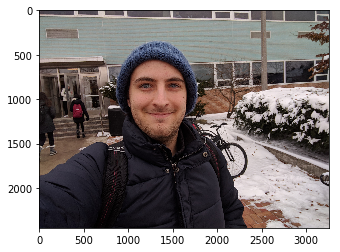
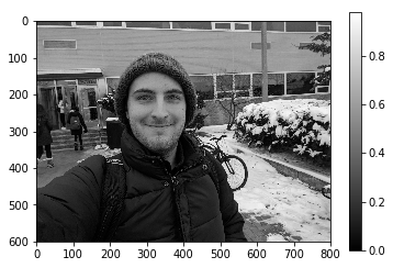
Goal: Detect a Human Face in a Selfie
I specifically chose selfies because the distance from the camera to the face would be relatively constant. This makes the recognition easier. I wasn’t sure how to deal with the challenge of drastically varying distances. Maybe I’ll attempt that in another tutorial, but for now we’ll stick with selfies.
1. Setup
The following packages are required for this tutorial:
- NumPy
- SciPy
- scikit-image
- matplotlib
Make sure to have these installed before continuing.
We start by importing the libraries…
import numpy as np
import matplotlib.pylab as plt
import matplotlib.image as mpimg
import scipy.ndimage
import skimage as ski
from matplotlib import patches
# Ignore if not using jupyter notebook or ipython
%matplotlib inline
# Ignore if not using jupyter notebook or ipython
%config IPCompleter.greedy=True
… and loading our target image.
fname = "eb-outside2.jpg"
img = mpimg.imread(fname)
plt.imshow(img)
<matplotlib.image.AxesImage at 0x112cbe4a8>
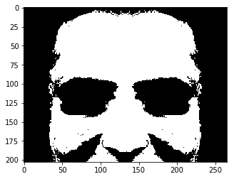
To perform the facial recognition, we use a mask. We will create a box the same size as the mask and move this box around the image. If the pixels inside the box are very similar to the mask, then it’s probably a face. This is an over-simplification of the procedure, but it’s the main idea. You can use the following image as a mask:
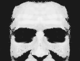
mask_img = mpimg.imread('filter_gray_3.jpg')
plt.imshow(mask_img, cmap='gray')
<matplotlib.image.AxesImage at 0x117996828>
2. Preparing the Images
We make sure our target image is scaled properly with respect to the mask. After doing some experimentation, I’ve found the following ratio to be ideal for selfies:
\[\frac{\text{target image height}}{\text{mask height}} \approx \frac{3}{1}\]target_scale = 600 / mask_img.shape[0] # 600 is based on experimentation
scale = img.shape[0] / mask_img.shape[0] # Get current ratio
scale_factor = target_scale / scale # Calculate nessecary scaling factor
img = ski.transform.rescale(img, scale_factor) # Perform Scale
You may receive the following warning:
UserWarning: The default multichannel argument (None) is deprecated.  Please specify either True or False explicitly.  multichannel will default to False starting with release 0.16.
UserWarning: The default mode, 'constant', will be changed to 'reflect' in skimage 0.15.
UserWarning: Anti-aliasing will be enabled by default in skimage 0.15 to avoid aliasing artifacts when down-sampling images.
Sci-kit will be pushing out an update soon and this warning will go away. It doesn’t affect our project so we can ignore it
Now we convert the images to grayscale. Let’s write a function to do this.
def to_grayscale(image, weights = np.c_[0.2989, 0.5870, 0.1140]):
    """
    Transforms a colour image to a greyscale image by
    taking the mean of the RGB values, weighted
    by the matrix weights
    """
    tile = np.tile(weights, reps=(image.shape[0],image.shape[1],1))
    avg = np.sum(tile * image, axis=2)  # Sum across z-axis
    return avg
Its computationally faster to process a grayscale image. By converting the image to grayscale, we eliminate 2 dimensions from our image. This is a result of mapping the RGB values to 1 grayscale value. The weights used are determined by the following grayscale equation:
\[Y' = 0.2989R' + 0.5870G' + 0.1140B'\]img_gray = to_grayscale(img)
plt.imshow(img_gray, cmap='gray')
plt.colorbar()
<matplotlib.colorbar.Colorbar at 0x11863b438>
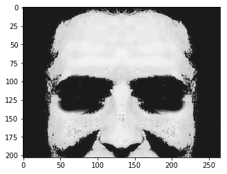
Let’s convert the mask to grayscale while also removing any noise in the mask. We want the mask to be consistent, so we will be using discrete values of 0 or 1 (black or white).
mask_img = to_grayscale(mask_img)
mask_img = (mask_img >= 150) * 1  # Remove low-brightness values to make mask more consistent
plt.imshow(mask_img, cmap='gray')
<matplotlib.image.AxesImage at 0x101d5c630>
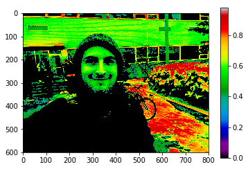
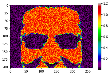
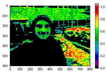
The same logic follows for the target image, however we want the detailed gradients. We multiply the original image by our filter to remove noise. We filter by all pixels larger than the average brightness.
avg_brightness = np.average(img_gray)
img_gray *= (img_gray > avg_brightness)  # Removes low-brightness noise
plt.imshow(img_gray, cmap='nipy_spectral')
plt.colorbar()
<matplotlib.colorbar.Colorbar at 0x111647da0>
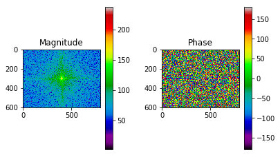
3. Moving to the frequency domain
The initial processing will take place in the frequency domain. You don’t need to understand the math behind this, but essentially we will be performing a Fast Fourier Transform (FFT) on the image. This represents the image as its constituent spatial frequency’s rather than normal pixels. When looking at FFT images, think of them more like a heat-map of frequencies.
Let’s start by defining a function to perform the FFT, and also perform a FFT shift. The shift just moves the high-frequency elements to the center of the image.
def to_fshift(img):
    return np.fft.fftshift(np.fft.fft2(img))
Let’s define the inverse function as well.
def to_ifft2(img_fshift):
    return np.abs(np.fft.ifft2(np.fft.ifftshift(img_fshift)))
We create another function to display the FFT image. We will plot the magnitude and phase of the FFT result. The magnitude has peaks at very sparse values, it makes sense for this to be in a log scale. We will use the following formula:
\[|f(j\omega)|_{db} = 20\log |f(j\omega)+1|\]def show_fft(img_fft):
'''
Displays the frequency-domain image.
This is done with 2 plots: Magnitude, and Phase.
The magnitude plot is in a dB scale(20*log)
The phase is plotted in units of degrees
'''
magnitude = 20*np.log(np.abs(img_fft)+ 1) # The magnitude of the image. Add 1 to deal with zeros
phase = np.angle(img_fft, deg=True) # Phase of the image (in degrees)
# Defines the subplot
fig, (ax0, ax1) = plt.subplots(nrows=1, ncols=2)
# Using tight layout to properly display plots
fig.tight_layout(pad=3)
# Plot magnitude
im_s = ax0.imshow(magnitude, cmap='nipy_spectral')
ax0.set_title('Magnitude')
fig.colorbar(im_s, ax=ax0)
# Plot phase
im_s = ax1.imshow(phase, cmap='nipy_spectral')
ax1.set_title('Phase')
fig.colorbar(im_s, ax=ax1)
We will need to display a spatial-domain image, given an FFT image. Let’s make a function to do that as well.
def show_ifft(img_fshift):
    img_ifft = to_ifft2(img_fshift)
    plt.imshow(img_ifft, cmap='nipy_spectral')
    plt.colorbar()
We will need a high-pass filter for this project. A simple way to do this is to use a low-pass filter, and subtract the result from the original input:
\[H_{pass} = T - L_{pass}\]def apply_lowpass(arr, w=None, h=None, r=None):
"""
Applys lowpass filter
"""
rows = np.shape(arr)[0]
cols = np.shape(arr)[1]
crow, ccol = rows//2, cols//2
lpass = arr.copy()
if w is None and h is None and r is None:
return None
elif r is None:
lpass[crow-h//2:crow+h//2,
ccol-w:ccol+w] = 0
elif w is None and h is None:
y,x = np.ogrid[-crow:rows-crow, -ccol:cols-ccol]
mask = x*x + y*y <= r*r
lpass[mask] = 0
return lpass
def apply_highpass(arr, w=None, h=None, r=None):
    return arr - apply_lowpass(arr, w, h, r)
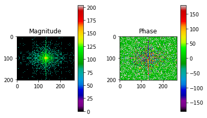
Now that we have our functions, we convert our spatial images to the frequency domain.
img_fshift = to_fshift(img_gray)
show_fft(img_fshift)
We filter out the low-magnitude frequencies. This makes our mask compressed, and smoother.
mask_fshift = to_fshift(mask_img)
mask_fshift *= (20*np.log(np.abs(mask_fshift)+1) > 75)  # 75 was determined from experimentation
# mask_fshift = apply_highpass(mask_fshift, r=25)
show_ifft(mask_fshift)
show_fft(mask_fshift)
We will now apply our mask in the frequency domain. Compared to the mask, this will amplify similar frequencies, and reduce the others.
mask_h,mask_w = mask_fshift.shape
img_h, img_w = img_fshift.shape
img_cy, img_cx = (img_h // 2, img_w // 2)
h0,w0 = (img_cy - mask_h // 2, img_cx - mask_w // 2)
h0,h1,w0,w1 = (h0,h0 + mask_h, w0,w0 + mask_w)
img_fshift[h0:h1, w0:w1] *= (mask_fshift != 0) * (img_fshift[h0:h1, w0:w1] != 0)
img_fshift = apply_highpass(img_fshift, r=100)
show_ifft(img_fshift)
show_fft(img_fshift)
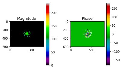
As you can see, the resulting target image is composed of far fewer frequencies than the original target image.
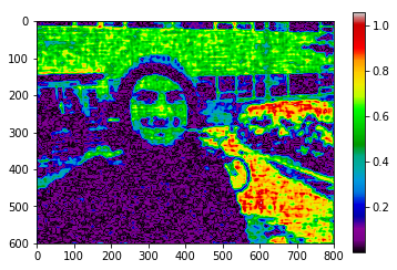
There is some resulting noise from this process. Let’s filter this out by removing pixels lower than the average brightness.
img_post_ifft = to_ifft2(img_fshift)
avg_brightness = np.average(img_post_ifft)
img_post_ifft *= (img_post_ifft > avg_brightness)
# img_post_ifft = img_post_ifft % 255
plt.imshow(img_post_ifft, cmap='nipy_spectral')
plt.colorbar()
<matplotlib.colorbar.Colorbar at 0x101e39588>
4. Finding the Face
Now that we have our image and mask formatted, and performed some preliminary processing, we can now apply the mask in the spatial domain. We start by defining the initial conditions for how our box will move around the image.
mask_h,mask_w = mask_fshift.shape  # The mask dimensions
img_h, img_w = img_fshift.shape  # The target image dimensions
# A dictionary to store the relative difference between the mask and box.
# It is keyed using the location
diffs = {}
# The resolution of the for-loop. It defines how much the 'box' moves each iteration
res = 10
# This buffer is used to store values with the smallest difference between the mask and box
buffer_size = res
# Define a matrix to be the buffer each row contains x, y, difference
center_arr = np.zeros((buffer_size, 3))  # 3D Coordinates, (x,y,diff)
# Convert the mask back to the spatial domain
mask_ifft = to_ifft2(mask_fshift)
# Remove noise
mask_ifft *= (mask_ifft > 0.4)
# Get the sum of the mask. This will be our reference
mask_sum = np.sum(mask_ifft)
5. The box function
Moving the box:
Our function will move a box around the processed target image, comparing itself to the mask_ifft image. Each iteration the box will translate in the \(x\) and \(y\) direction by the following ratio:
\(\text{Given $i_n$ and $j_n$ is the current position of the box:} \\
i_n = i_{n-1} + \frac{\text{mask height}}{\text{resolution}} \\
j_n = j_{n-1} + \frac{\text{mask height}}{\text{resolution}}\)
Applying the Mask:
There are a few conditions we must consider when applying our mask. Let’s define our function \(B_{\text{diff}}(B,M)\) where \(B\) is the matrix (image) of the box and \(M\) is the matrix (image) of the mask. \(B_{\text{diff}}(B,M)\) maps the set of boxes and masks to the set of matrices consisting of the differences between the two. \(B_{\text{diff}}(B,M)\) must be one-to-one and continuous for all \(B\) and \(M\). Given our function is defined as continuous and one-to-one, the intermediate value theroem applies. This implies that only the boundary cases need consideration while building \(B_{\text{diff}}(B, M)\). Additionally, the domain of \(B_{\text{diff}}(B,M)\) are discrete values of \(0\) or \(1\). Moreover, \(M\) remains constant as the box translates around the target image.
Given all these constraints, there are two boundary cases to consider: \(B\) is a matrix of \(1\)’s, and \(B\) is a matrix of \(0\)’s.
Given \(B_1 = \begin{bmatrix} 1 & 1 & \dots \\ \vdots & \ddots & \\ 1 & 1 & 1 \\ \end{bmatrix}\) where \(B\) and \(M\) are \(a \times b\) matrices, we must develop an equation such that \(\sum B_{\text{diff}}(B_1,M) \not= \sum(M)\) \(\begin{align} R &= M \odot B \\ R' &= M -2M \odot B + B \\ B_{\text{diff}}(B,M) &= R - R' = \sum_{i=0}^{a}\sum_{j=0}^{b}(r_{ij}) - \sum_{i=0}^{a}\sum_{j=0}^{b}(r'_{ij}) \\ R_{B_1} &= M \odot B_1 = M \\ R'_{B_1} &= M -2M \odot B_1 + B_1 = M - 2M + B_1 = B_1 - M \\ B_{\text{diff}}(B_1,M) &= R_{B_1} - R'_{B_1} = M - (B_1 - M) = 2M - B_1 \\ \sum B_{\text{diff}}(B_1,M) &= \sum(2M - B_1) \not= \sum(M) \end{align}\)
Given \(B_0 = \begin{bmatrix} 0 & 0 & \dots \\ \vdots & \ddots & \\ 0 & 0 & 0 \\ \end{bmatrix}\) where \(B\) and \(M\) are \(a \times b\) matrices, we must develop an equation such that \(\sum B_{\text{diff}}(B_0,M) \not= \sum(M)\) \(\begin{align} R &= M \odot B \\ R' &= M -2M \odot B + B \\ B_{\text{diff}}(B,M) &= R - R' = \sum_{i=0}^{a}\sum_{j=0}^{b}(r_{ij}) - \sum_{i=0}^{a}\sum_{j=0}^{b}(r'_{ij}) \\ R_{B_0} &= M \odot B_0 = B_0 \\ R'_{B_0} &= M -2M \odot B_0 + B_0 = M - B_0 + B_0 = M \\ B_{\text{diff}}(B_0,M) &= R_{B_0} - R'_{B_0} = B_0 - M = -M\\ \sum B_{\text{diff}}(B_0,M) &= \sum(-M) \not= \sum(M) \end{align}\)
This function is written as follows:
for h in range(0, img_h - mask_h, mask_h // res):
    for w in range(0, img_w - mask_w, mask_w // res):
        # Creates Box
        box = img_post_ifft[h:h+mask_h, w:w+mask_w].copy()
        # All elements that ARE in mask and NOT zero
        box_diff = (mask_ifft != 0) * (box != 0)
        # All elements that are NOT in mask and ARE zero
        box_diff_inv = (mask_ifft == 0) * (box == 0)
        # Subtract the box_diff with it's inverse
        box_sum = np.sum(box_diff) - np.sum(box_diff_inv)
        key = (h,w)
        # Write the ratio to the dictionary
        diffs[key] = box_sum/mask_sum
We need to find the the coordinates of the box with the smallest difference between it and the mask. We will store these values in the buffer.
Based on our function \(B_{\text{diff}}(B,M)\), we can use the following ratio to determine the likeness between the box and our mask:
\[\frac{B_{\text{diff}}(B,M)}{\sum(M)} \\\]This ratio has the following property:
\[\frac{B_{\text{diff}}(M,M)}{\sum(M)} = \frac{\sum(M)}{\sum(M)} = 1 \\\]This allows us to determine how much the box and mask differ.
for key,val in diffs.items():
    for i,m in enumerate(center_arr):
        if abs(val-1) < m[-1] or m[-1] == 0:
            center_arr[i,-1] = val
            center_arr[i,:-1] = key[::-1]  # center_arr in x,y
            center_arr[i,1] += mask_h // 4
            break
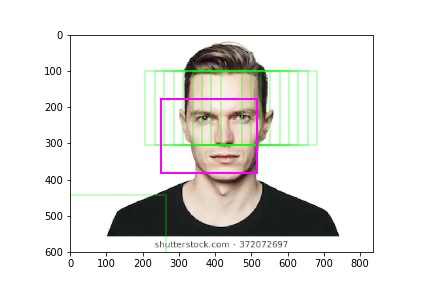
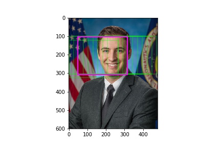
Finally we plot the box’s which differ the least from the mask onto the original target image.
We accomplish this by taking the weighted average of the buffer’s coordinates. The weight is determined by the ratio between the box and mask.
fig, ax = plt.subplots(1)
for c in center_arr[:,:-1]:
    ax.add_patch(patches.Rectangle(c, width=mask_w, height=mask_h, color=(0,1,0,0.25), linewidth=2, fill=False))
# avg_c = center_arr[np.argmin(center_arr[:,-1]),:-1]
avg_c = np.average(center_arr[:,:-1], axis=0, weights=center_arr[:,-1])
ax.add_patch(patches.Rectangle(avg_c, width=mask_w, height=mask_h, color=(1,0,1), linewidth=2, fill=False))
ax.imshow(img)
fig.savefig('{}_result.jpg'.format(fname[:-4]))

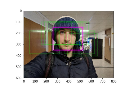
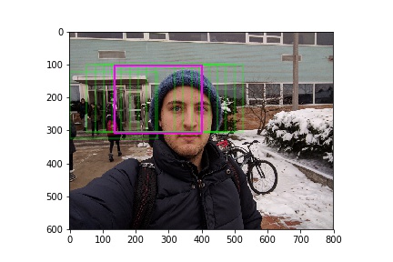
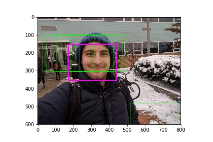
Results
Below are a few other successful results: